```{r setup, include=FALSE, message = FALSE}
library(methods)
knitr::opts_chunk$set(echo = TRUE, comment = "")
library(methods)
library(ggplot2)
library(ms.lesion)
library(neurobase)
library(extrantsr)
library(scales)
```
## MS Lesion
Let's reset and read in the T1 image from a MS lesion data set:
```{r reading_in_image, eval = FALSE}
t1 = neurobase::readnii("training01_01_t1.nii.gz")
t1[ t1 < 0 ] = 0
```
```{r reading_in_image_run, echo = FALSE}
t1 = neurobase::readnii("../training01_01_t1.nii.gz")
t1[ t1 < 0 ] = 0
```
## Overall Pipeline
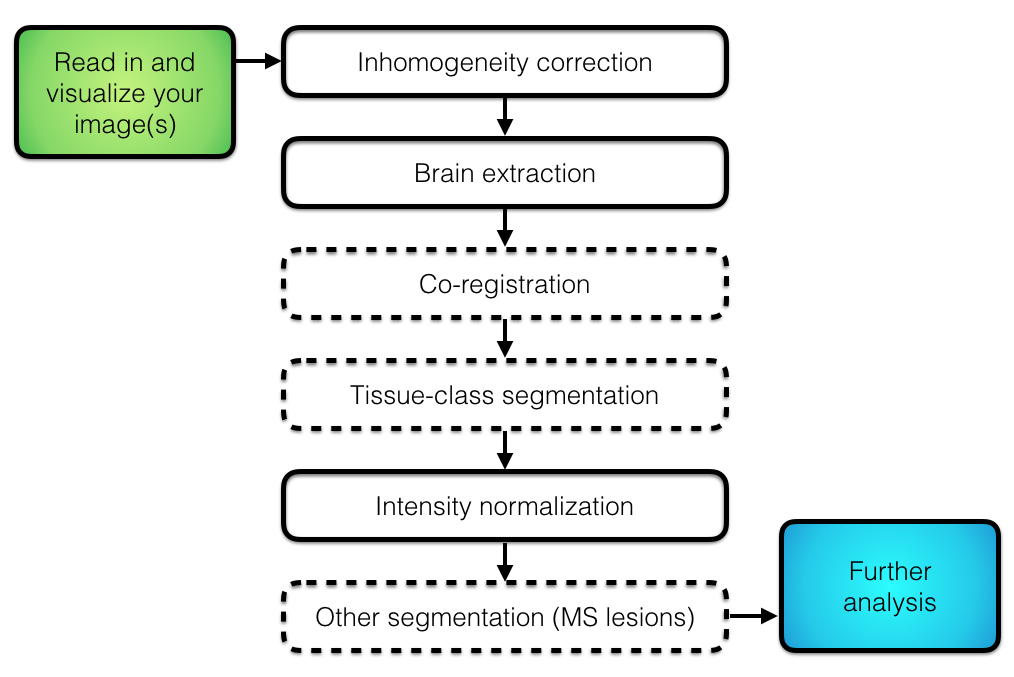 ## Inhomogeneity correction
- Scans can have nonuniform intensities throughout the brain
- Usually low frequency - smooth over the brain (assumed)
- Referred to as bias, bias field, or inhomogeneity
## Inhomogeneity correction
- Scans can have nonuniform intensities throughout the brain
- Usually low frequency - smooth over the brain (assumed)
- Referred to as bias, bias field, or inhomogeneity
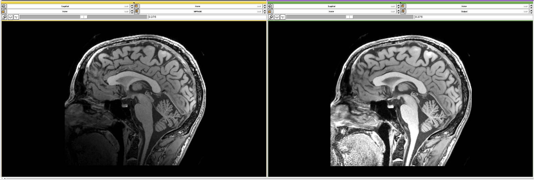 Image From https://www.slicer.org/w/images/7/77/MRI_Bias_Field_Correction_Slicer3_close_up.png
## Image Data
It's hard to see subtler bias fields, but sometimes they can be seen visually.
```{r ortho2_show}
ortho2(robust_window(t1))
```
## Image Data
```{r ortho2_show_flair, eval = FALSE}
flair = neurobase::readnii("training01_01_flair.nii.gz")
ortho2(robust_window(flair))
```
```{r ortho2_run_flair, echo = FALSE}
flair = neurobase::readnii("../training01_01_flair.nii.gz")
flair[ flair < 0 ] = 0
flair = drop_empty_dim(flair > 50, other.imgs = flair)
flair = flair$other.imgs
ortho2(robust_window(flair))
```
## Image Data: Lightbox
```{r lightbox}
image(robust_window(t1), useRaster = TRUE)
```
## N4 Inhomogeneity Correction
We will use N4: Improved N3 Bias Correction [@tustison_n4itk_2010].
The model assumed in the N4 is:
$$
v(x) = u(x)f(x) + n(x)
$$
- $v$ is the given image
- $u$ is the uncorrupted image
- $f$ is the bias field
- $n$ is the noise (assumed to be independent and Gaussian)
- $x$ is a location in the image
## N4 Inhomogeneity Correction
The data is log-transformed and assuming a noise-free scenario, we have:
$$
\log(v(x)) = \log(u(x)) + \log( f(x) )
$$
- N4 uses a B-spline approximation of the bias field
- It iterates until a convergence criteria is met
- when the updated bias field is the same as the last iteration
- It outputs the data back in the original units (not log-transformed)
## Bias Field Correction
Here we will use the `bias_correct` function in `extrantsr`, which calls `n4BiasFieldCorrection` from `ANTsR`.
You can pass in the image:
```{r bc_show, message = FALSE, eval = FALSE}
library(extrantsr)
bc_t1 = bias_correct(file = t1, correction = "N4")
```
```{r bc_run, echo = FALSE}
out_fname = "../output/training01_01_t1_n4.nii.gz"
if (!file.exists(out_fname)) {
bc_t1 = bias_correct(file = t1, correction = "N4")
} else {
bc_t1 = readnii(out_fname)
}
```
or the filename (but negatives are in there):
```{r, eval = FALSE}
bc_t1 = bias_correct(file = "training01_01_t1.nii.gz", correction = "N4")
```
## Visualizing Bias Field Correction
Here we take the ratio of the images and overlay it on the original image:
```{r ratio_plot}
ratio = t1 / bc_t1; ortho2(t1, ratio)
```
```{r making_scales, echo = FALSE}
library(scales)
in_mask = (ratio < 0.999 | ratio > 1.0001) & ratio != 0
# get the quantiles
quantiles = quantile(ratio[ in_mask ], na.rm = TRUE,
probs = seq(0, 1, by = 0.1) )
quantiles = unique(quantiles)
# get a diverging gradient palette
fcol = scales::brewer_pal(type = "div", palette = "Spectral")(10)
# need one fewer color than breaks/quantiles
colors = gradient_n_pal(fcol)(seq(0,1, length = length(quantiles) - 1))
colors = scales::alpha(colors, 0.5) # colors are created
```
## Visualizing Bias Field Correction
We are breaking the ratio into quantiles:
```{r better_ratio_plot}
ortho2(t1, ratio, col.y = colors, ybreaks = quantiles, ycolorbar = TRUE)
```
## Conclusions
- Inhomogeneity correction is one of the first steps of most structural MRI pipelines
- Inhomogeneity can cause problems for other methods/segmentation
- Corrections try to make tissues of the same class to have similar intensities
- Use the `extrantsr` `bias_correct` function
- There is also `fsl_biascorrect` from `fslr` (not as effective in our experience)
- You may also want to run corrections after skull stripping on the brain only
- this is possible with the result after the brain extraction lecture
- correction before skull-stripping may be necessary and can improve after correction
## Website
http://johnmuschelli.com/imaging_in_r
## References
Image From https://www.slicer.org/w/images/7/77/MRI_Bias_Field_Correction_Slicer3_close_up.png
## Image Data
It's hard to see subtler bias fields, but sometimes they can be seen visually.
```{r ortho2_show}
ortho2(robust_window(t1))
```
## Image Data
```{r ortho2_show_flair, eval = FALSE}
flair = neurobase::readnii("training01_01_flair.nii.gz")
ortho2(robust_window(flair))
```
```{r ortho2_run_flair, echo = FALSE}
flair = neurobase::readnii("../training01_01_flair.nii.gz")
flair[ flair < 0 ] = 0
flair = drop_empty_dim(flair > 50, other.imgs = flair)
flair = flair$other.imgs
ortho2(robust_window(flair))
```
## Image Data: Lightbox
```{r lightbox}
image(robust_window(t1), useRaster = TRUE)
```
## N4 Inhomogeneity Correction
We will use N4: Improved N3 Bias Correction [@tustison_n4itk_2010].
The model assumed in the N4 is:
$$
v(x) = u(x)f(x) + n(x)
$$
- $v$ is the given image
- $u$ is the uncorrupted image
- $f$ is the bias field
- $n$ is the noise (assumed to be independent and Gaussian)
- $x$ is a location in the image
## N4 Inhomogeneity Correction
The data is log-transformed and assuming a noise-free scenario, we have:
$$
\log(v(x)) = \log(u(x)) + \log( f(x) )
$$
- N4 uses a B-spline approximation of the bias field
- It iterates until a convergence criteria is met
- when the updated bias field is the same as the last iteration
- It outputs the data back in the original units (not log-transformed)
## Bias Field Correction
Here we will use the `bias_correct` function in `extrantsr`, which calls `n4BiasFieldCorrection` from `ANTsR`.
You can pass in the image:
```{r bc_show, message = FALSE, eval = FALSE}
library(extrantsr)
bc_t1 = bias_correct(file = t1, correction = "N4")
```
```{r bc_run, echo = FALSE}
out_fname = "../output/training01_01_t1_n4.nii.gz"
if (!file.exists(out_fname)) {
bc_t1 = bias_correct(file = t1, correction = "N4")
} else {
bc_t1 = readnii(out_fname)
}
```
or the filename (but negatives are in there):
```{r, eval = FALSE}
bc_t1 = bias_correct(file = "training01_01_t1.nii.gz", correction = "N4")
```
## Visualizing Bias Field Correction
Here we take the ratio of the images and overlay it on the original image:
```{r ratio_plot}
ratio = t1 / bc_t1; ortho2(t1, ratio)
```
```{r making_scales, echo = FALSE}
library(scales)
in_mask = (ratio < 0.999 | ratio > 1.0001) & ratio != 0
# get the quantiles
quantiles = quantile(ratio[ in_mask ], na.rm = TRUE,
probs = seq(0, 1, by = 0.1) )
quantiles = unique(quantiles)
# get a diverging gradient palette
fcol = scales::brewer_pal(type = "div", palette = "Spectral")(10)
# need one fewer color than breaks/quantiles
colors = gradient_n_pal(fcol)(seq(0,1, length = length(quantiles) - 1))
colors = scales::alpha(colors, 0.5) # colors are created
```
## Visualizing Bias Field Correction
We are breaking the ratio into quantiles:
```{r better_ratio_plot}
ortho2(t1, ratio, col.y = colors, ybreaks = quantiles, ycolorbar = TRUE)
```
## Conclusions
- Inhomogeneity correction is one of the first steps of most structural MRI pipelines
- Inhomogeneity can cause problems for other methods/segmentation
- Corrections try to make tissues of the same class to have similar intensities
- Use the `extrantsr` `bias_correct` function
- There is also `fsl_biascorrect` from `fslr` (not as effective in our experience)
- You may also want to run corrections after skull stripping on the brain only
- this is possible with the result after the brain extraction lecture
- correction before skull-stripping may be necessary and can improve after correction
## Website
http://johnmuschelli.com/imaging_in_r
## References